3.1 Exercises

Q1: Draw a boxplot of hwy for each value of cyl, without turning cyl into a factor. What extra aesthetic do you need to set?

A: We need to set group aesthetic:

ggplot(mpg, aes(cyl, hwy, group = cyl)) +
  geom_boxplot()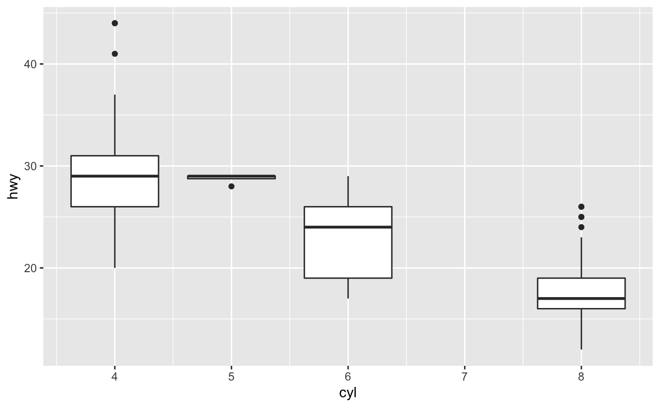

Q2: Modify the following plot so that you get one boxplot per integer value of displ.

ggplot(mpg, aes(displ, cty)) + 
  geom_boxplot()
#> Warning: Continuous x aesthetic -- did you forget aes(group=...)?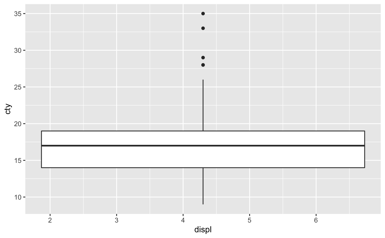

A: As the warning hints us, we have to set the group aesthetic:

ggplot(mpg, aes(displ, cty, group = displ)) + 
  geom_boxplot()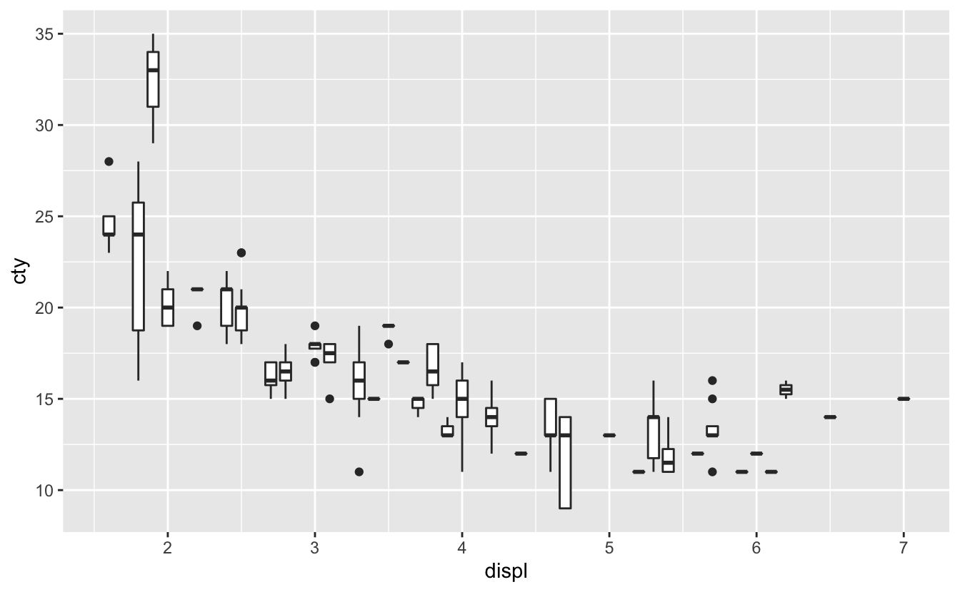

Q3: When illustrating the difference between mapping continuous and discrete colours to a line, the discrete example needed aes(group = 1). Why? What happens if that is omitted? What’s the difference between aes(group = 1) and aes(group = 2)? Why?

A: First, lets remove the group aesthetic:

df <- data.frame(x = 1:3, y = 1:3, colour = c(1, 3, 5))

ggplot(df, aes(x, y, colour = factor(colour))) + 
  geom_line(size = 2) +
  geom_point(size = 5)
#> geom_path: Each group consists of only one observation. Do you need to adjust
#> the group aesthetic?

ggplot(df, aes(x, y, colour = colour)) + 
  geom_line(size = 2) +
  geom_point(size = 5)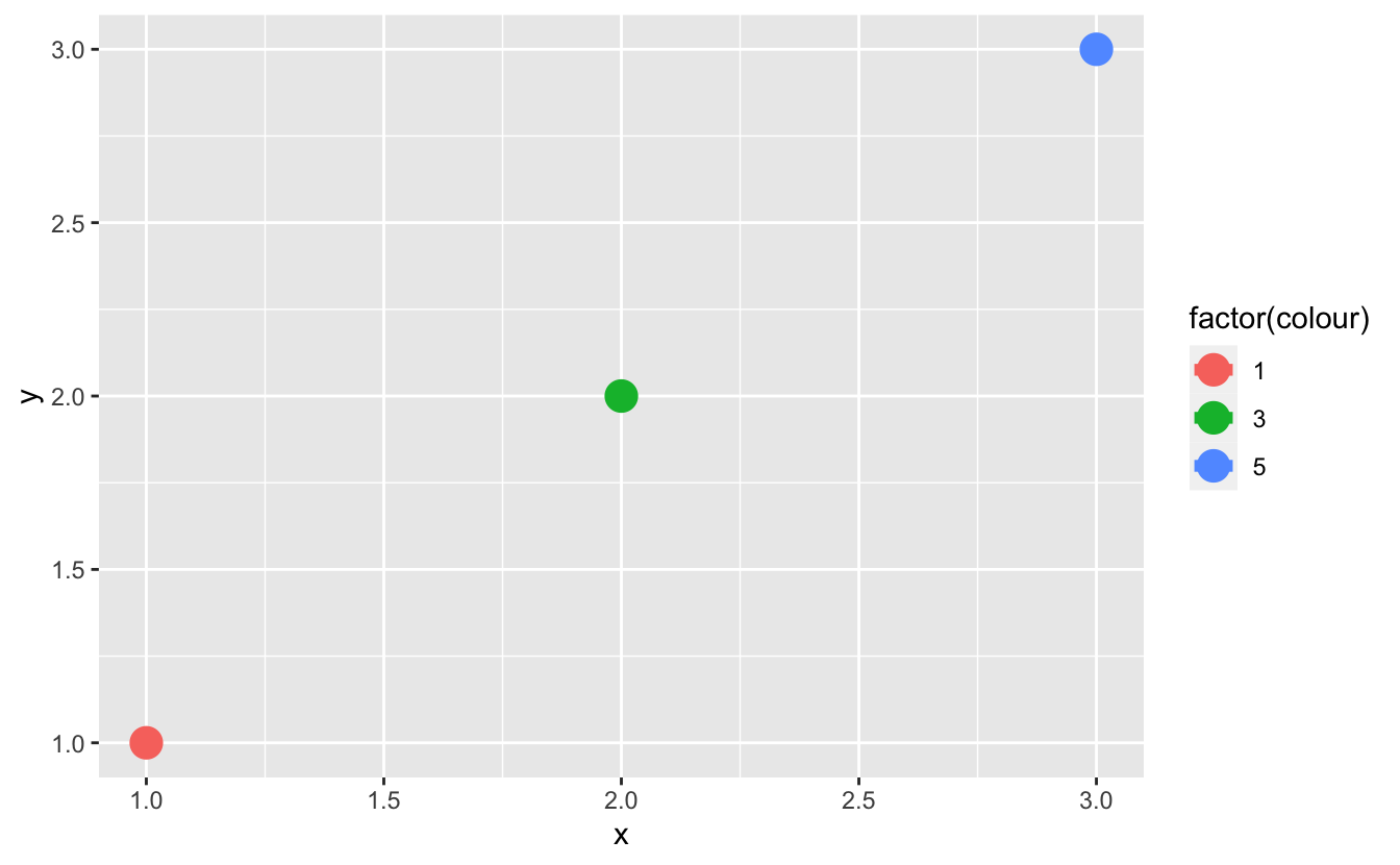

Now let’s use aes(group = 2):

ggplot(df, aes(x, y, colour = factor(colour))) + 
  geom_line(aes(group = 2), size = 2) +
  geom_point(size = 5)

ggplot(df, aes(x, y, colour = colour)) + 
  geom_line(aes(group = 2), size = 2) +
  geom_point(size = 5)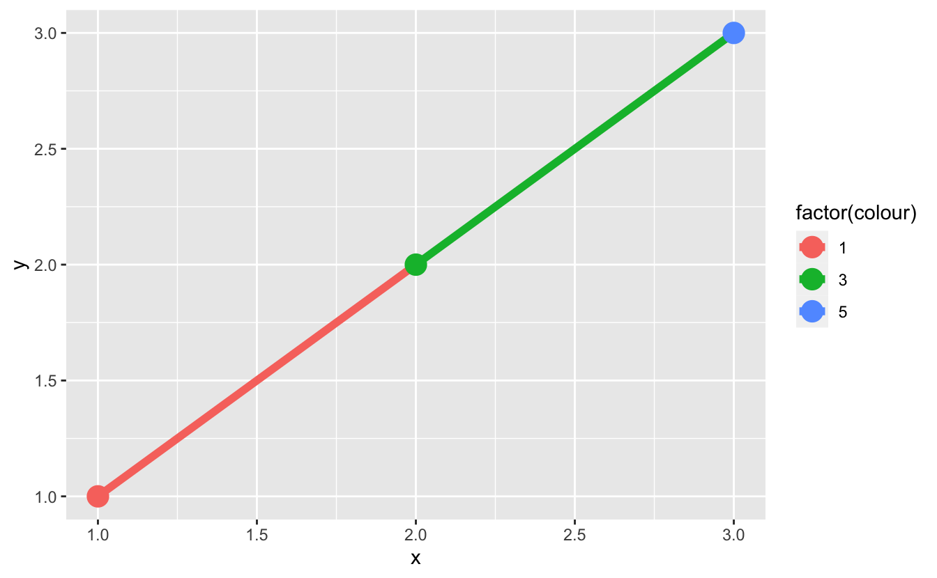

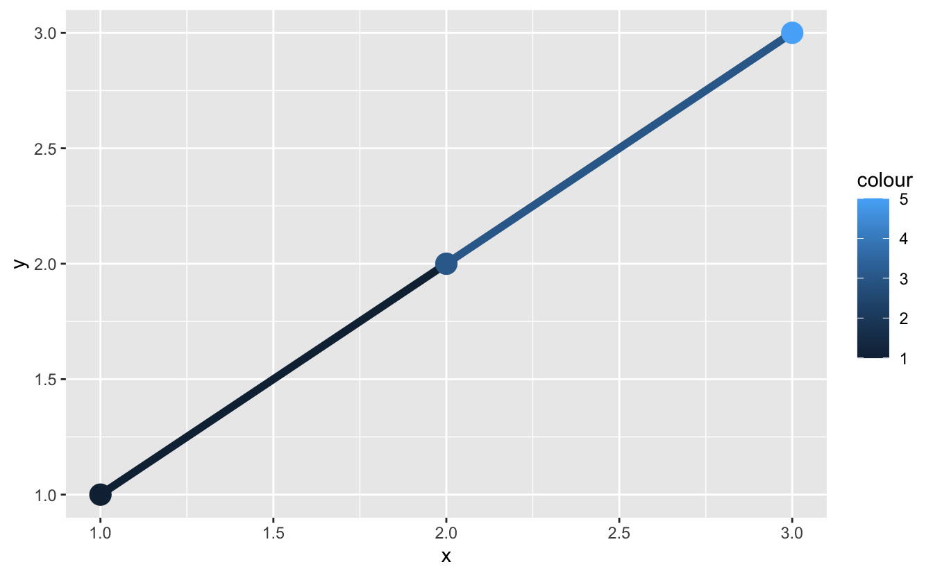
If we map a categorical variable to the color aesthetic, geom_line() connects (group) the observations in each level of the variable. In the first case, there is only one observation in each group so, specifying the groups manually makes these points connected (and in the second case, we can notice that the value of the group aesthetic doesn’t matter).

Q4: How many bars are in each of the following plots?

ggplot(mpg, aes(drv)) + 
  geom_bar()

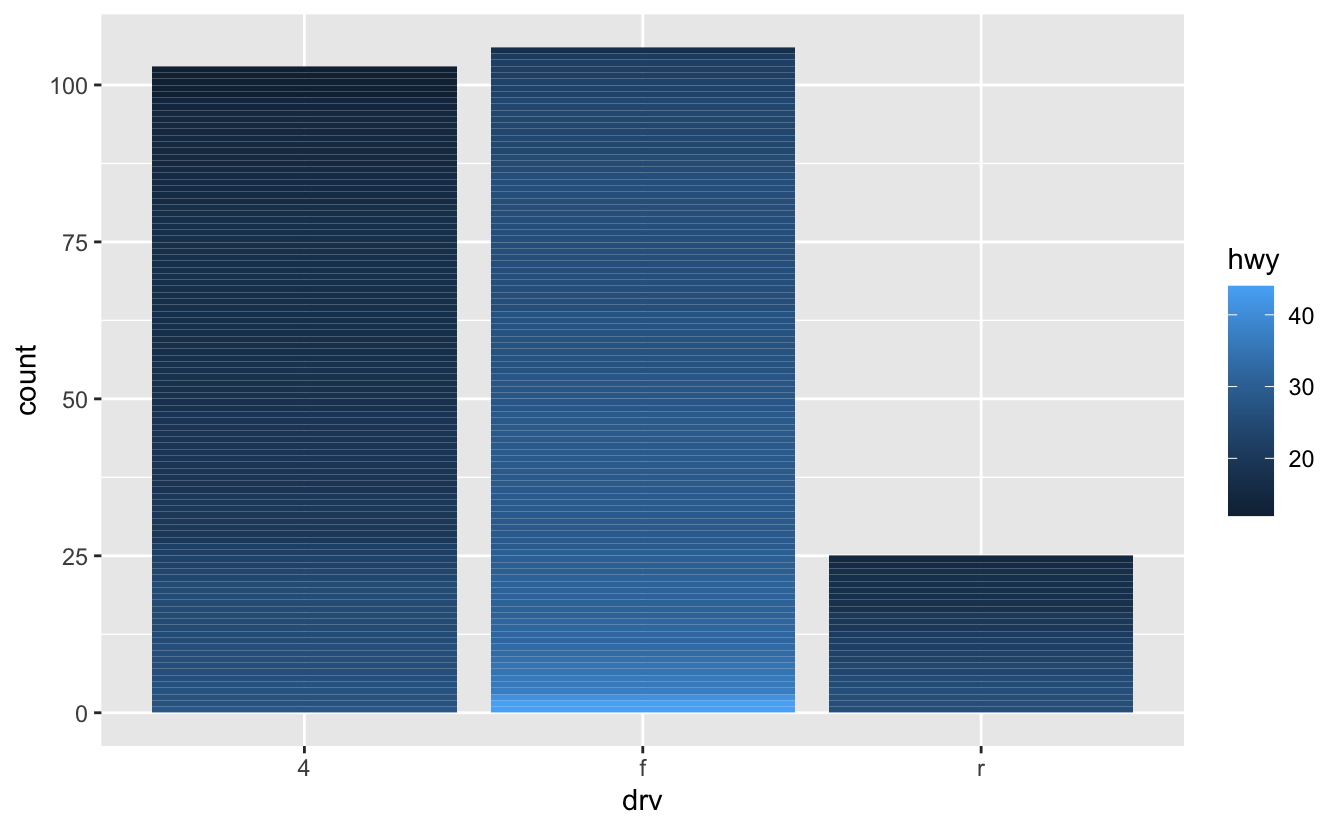
ggplot(mpg, aes(drv, fill = hwy, group = hwy)) + 
  geom_bar()

mpg2 <- mpg %>% arrange(hwy) %>% mutate(id = seq_along(hwy)) 
ggplot(mpg2, aes(drv, fill = hwy, group = id)) + 
  geom_bar()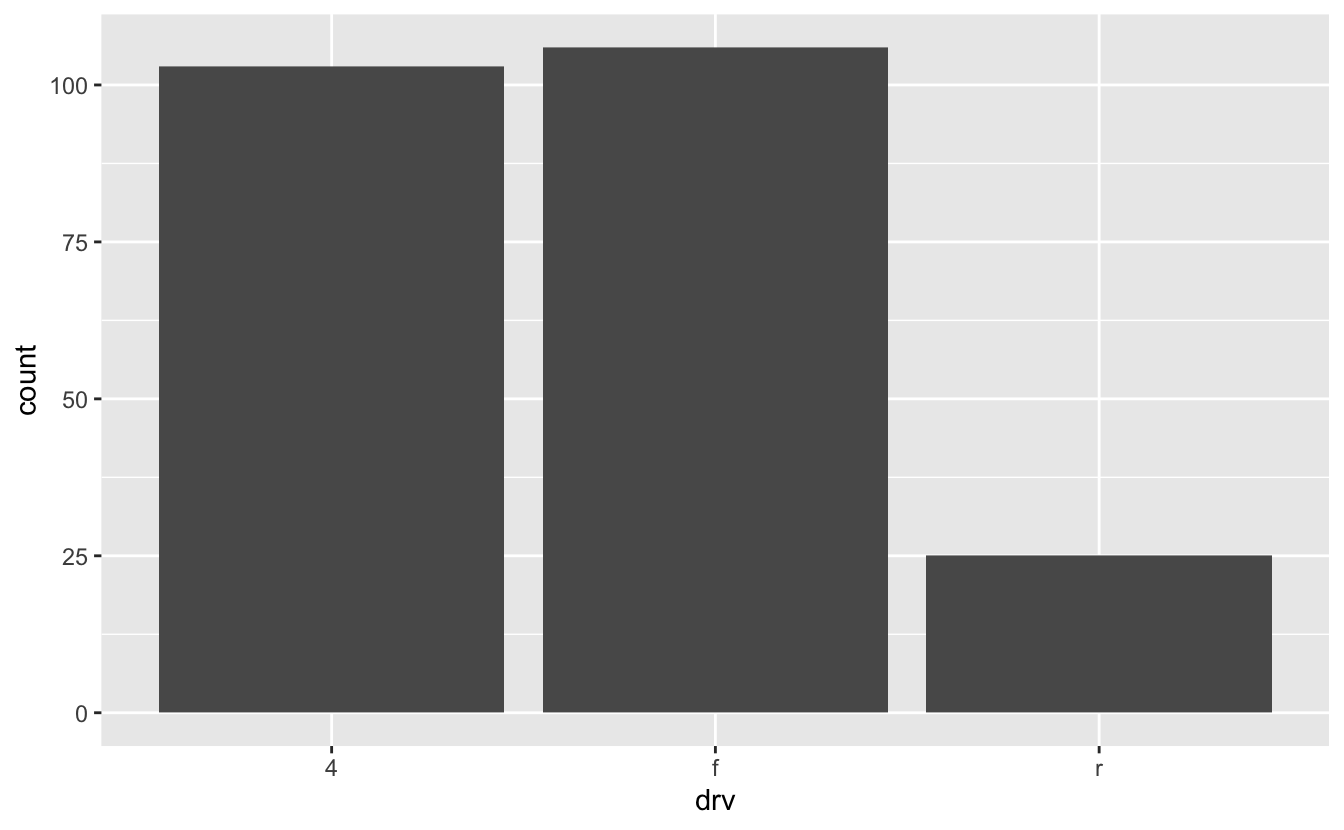

(Hint: try adding an outline around each bar with colour = "white")

A: We can use colour = "white", but it’s still hard to count the number of bars. We can use dplyr to find the number of bars:

ggplot(mpg, aes(drv)) + 
  geom_bar(color = "white")


mpg %>%
  select(drv) %>%
  unique() %>%
  group_by(drv) %>%
  count()
#> # A tibble: 3 x 2
#> # Groups:   drv [3]
#>   drv       n
#>   <chr> <int>
#> 1 4         1
#> 2 f         1
#> 3 r         1

ggplot(mpg, aes(drv, fill = hwy, group = hwy)) + 
  geom_bar(color = "white")

mpg %>% 
  select(drv, hwy) %>% 
  unique() %>% 
  count(drv)
#> # A tibble: 3 x 2
#>   drv       n
#>   <chr> <int>
#> 1 4        15
#> 2 f        20
#> 3 r        11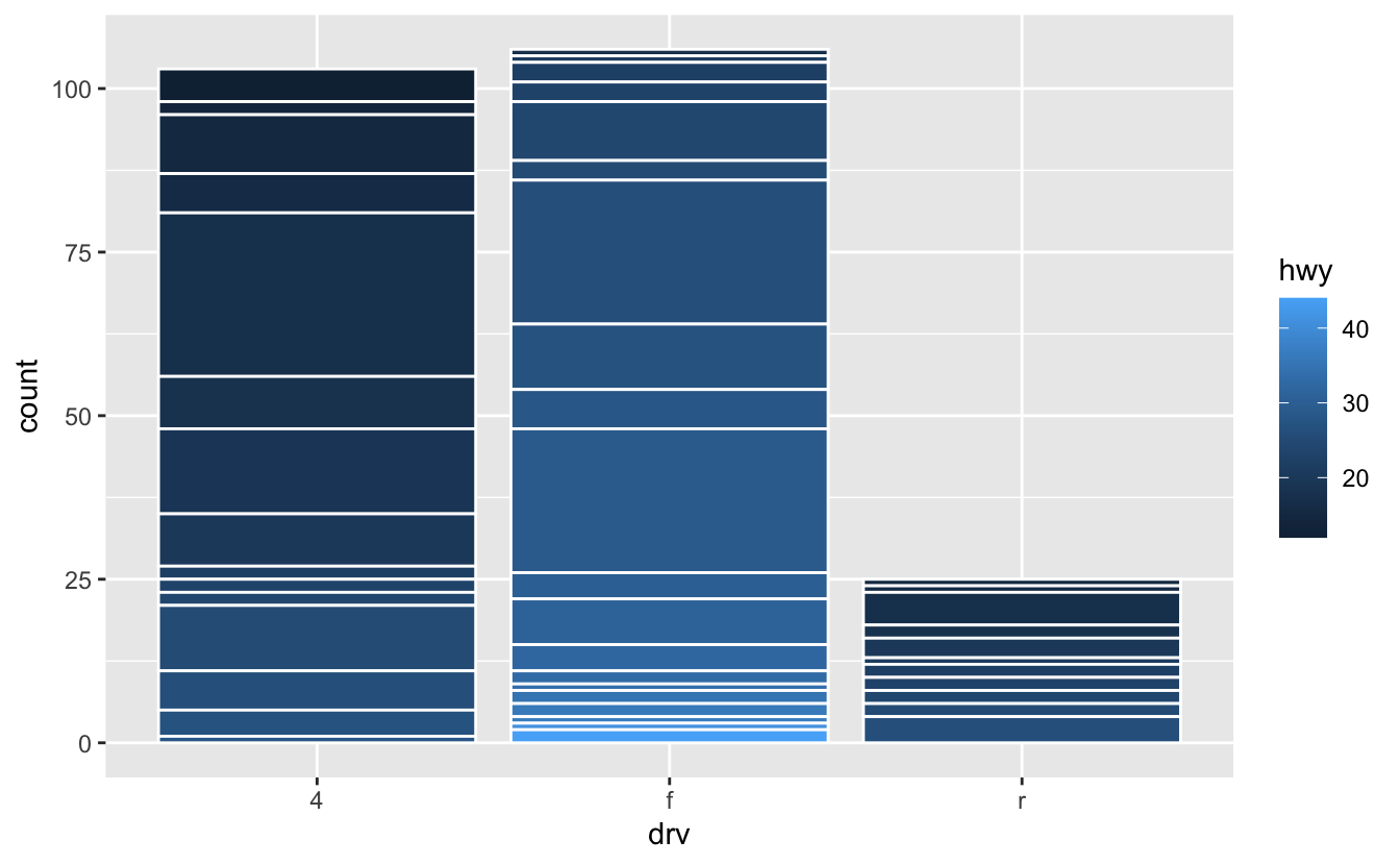

mpg2 <- mpg %>% arrange(hwy) %>% mutate(id = seq_along(hwy))

ggplot(mpg2, aes(drv, fill = hwy, group = id)) + 
  geom_bar(color = "white")


mpg2 %>%
  select(drv, hwy, id) %>%
  unique() %>%
  count(drv)
#> # A tibble: 3 x 2
#>   drv       n
#>   <chr> <int>
#> 1 4       103
#> 2 f       106
#> 3 r        25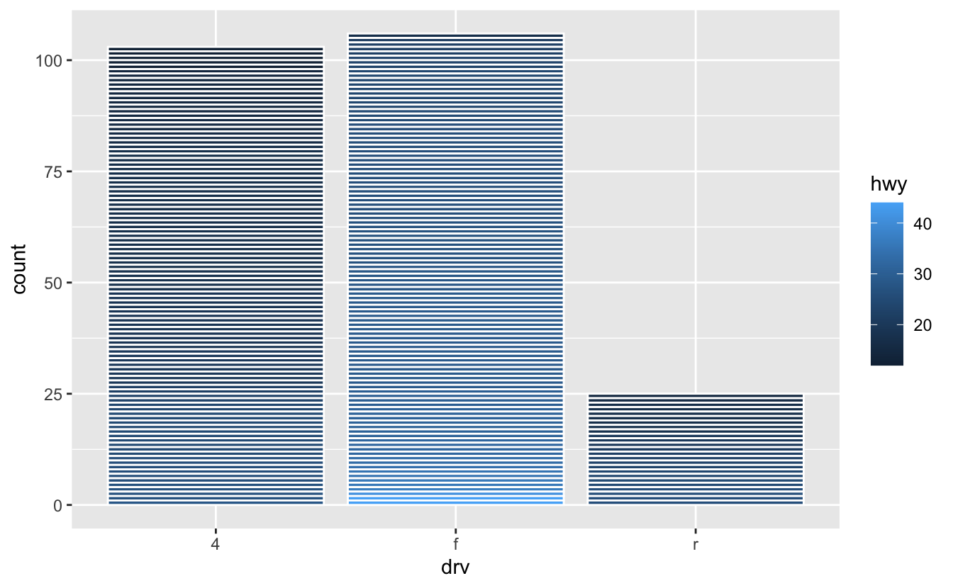

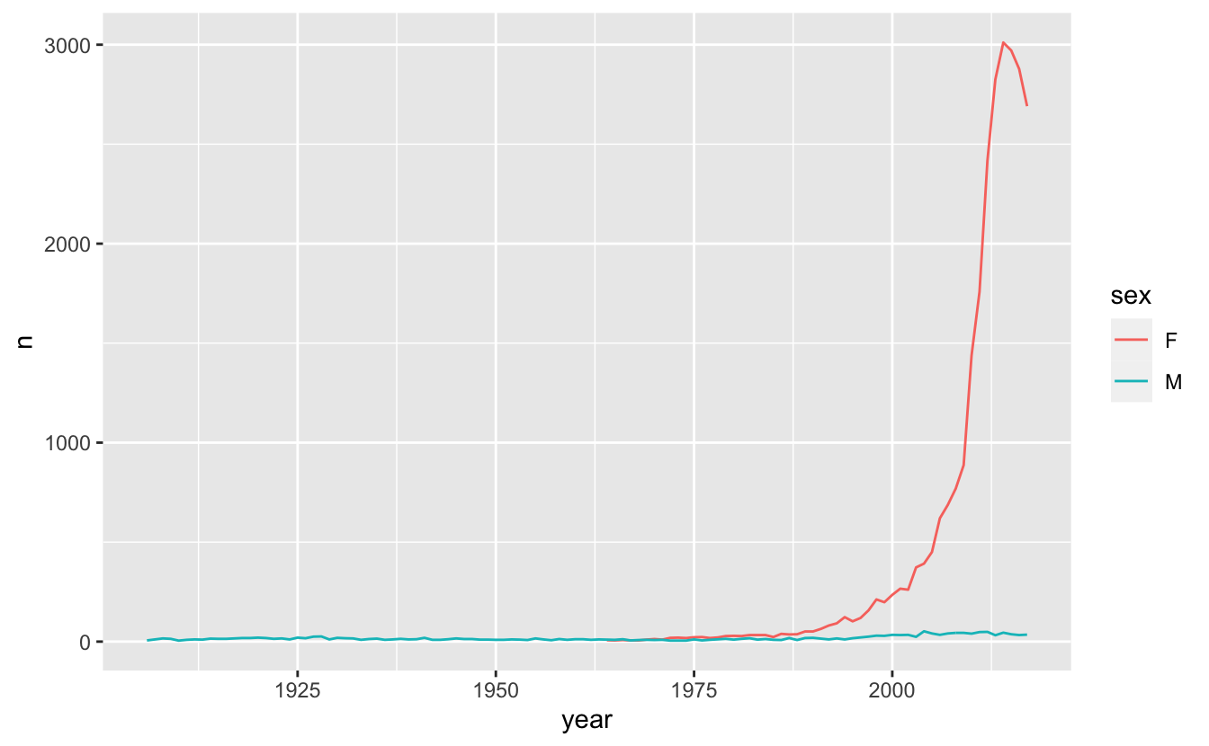
Q5: Install the babynames package. It contains data about the popularity of babynames in the US. Run the following code and fix the resulting graph. Why does this graph make me unhappy?

hadley <- filter(babynames, name == "Hadley")
ggplot(hadley, aes(year, n)) + 
  geom_line()

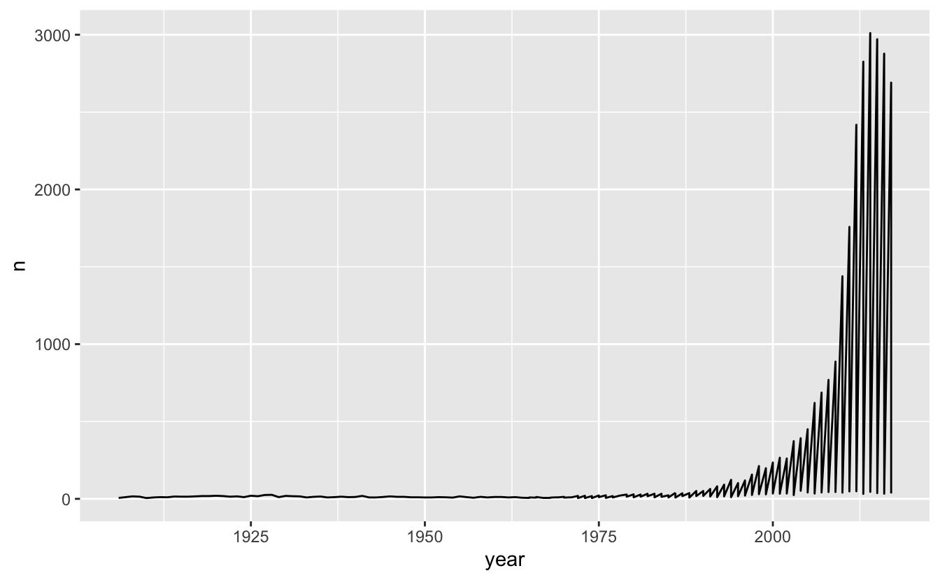
A: We want to see the growth of the newborn babies with the name called Hadley. If we take a look at the data, we can notice that there are 2 levels for the sex variable:

hadley <- filter(babynames, name == "Hadley")
levels(as.factor(hadley$sex))
#> [1] "F" "M"

There is two way to fix this problem: using group aesthetic or using colour aesthetic:

ggplot(hadley, aes(year, n, colour = sex)) + 
  geom_line()